matlab is a powerful tool on which we can perform or apply different algorithms. this is very much powerful almost used everywhere in the industry, without this nothing is possible and due to this powerfulness this tool is used also in industry and military for performing different tasks and projects and this is the reason that is also used in the aero space industry for manufacturing different types of planes and their control.
Question # 01
% Program P1_7 % Generate the input signal
clear all; close all; clc;
n =0:100;
s1 = cos(2*pi*0.05*n); % A low frequency sinusoid
s2 = cos(2*pi*0.47*n); % A high frequency sinusoid
x = s1+s2; % Implementation of the moving average filter
M = input('Desired length of the filter = ');
num = ones(1,M);
y = filter(num,1,x)/M; % Display the input and output signals
subplot(2,2,1);
plot(n,s1);
axis([0, 100, -2, 2]);
xlabel('Time index n');
ylabel('Amplitude');
title('Signal # 1');
subplot(2,2,2);
plot(n,s2);
axis([0, 100, -2, 2]);
xlabel('Time index n'); ylabel('Amplitude');title('Signal # 2');
subplot(2,2,3);
plot(n,x); axis([0, 100, -2, 2]);
xlabel('Time index n'); ylabel('Amplitude'); title('Input Signal');
subplot(2,2,4); plot(n,y); axis([0, 100, -2, 2]);
xlabel('Time index n'); ylabel('Amplitude'); title('Output Signal');
In Command Window
Desired length of the filter = 2
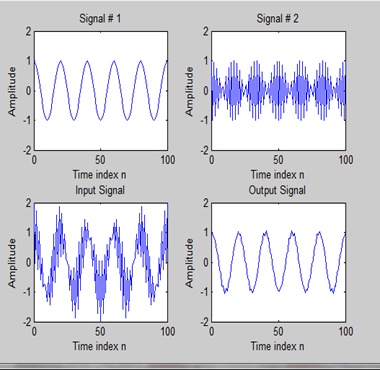
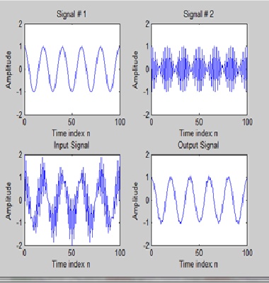
As this bhave as a low pass filter so its allow the low frequency signal S1 and suppressed the high frequency component as S2
Question #02
% Program P1_7 % Generate the input signal
clear all; close all; clc;
n =0:100;
s1 = cos(2*pi*0.05*n); % A low frequency sinusoid
s2 = cos(2*pi*0.47*n); % A high frequency sinusoid
x = s1+s2 % Implementation of the moving average filter
y1=0.5*([x 0]+[0 x])
y2=0.5*([x 0]-[0 x])
subplot(4,1,1)
stem(y1)
subplot(4,1,2)
stem(y2)
subplot(4,1,3)
stem(s1)
subplot(4,1,4)
stem(s2)
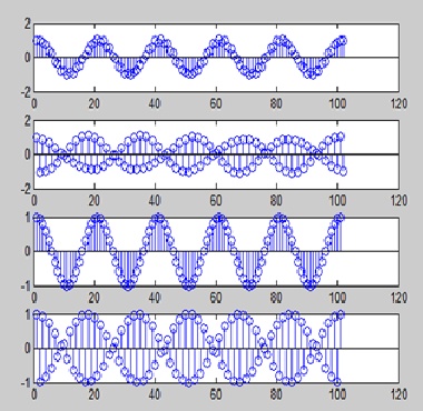
By using Y1 and Y2 I recover s1 and s2…!
Question #3
(a)
In Command Window
Desired length of the filter = 3
(b)
In Command Window
Desired length of the filter = 5
(a)
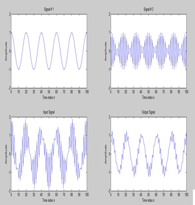
(b)by increasing the frequency high and by incresasing the value of M filter its supressed yhe high frequencies
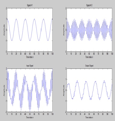
Question #4
Frequency of s1=0.05
Frequency of s2 = 0.47
s1 = cos(2*pi*0.05*n);
s2 = cos(2*pi*0.47*n);
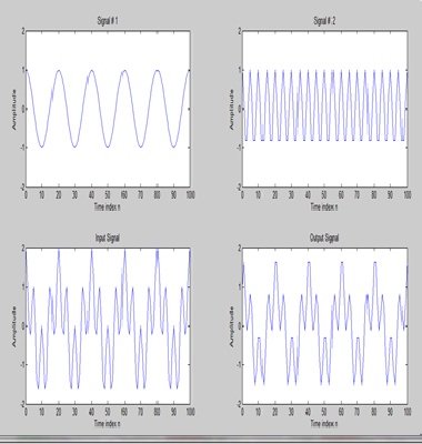
Frequency of s1 = 0.10
Frequency of s2 =0.90
s1 = cos(2*pi*0.10*n);
s2 = cos(2*pi*0.90*n);
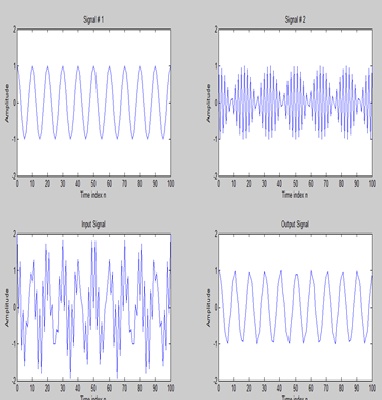
Frequency of s1=0.30
Frequency of s2=0.47
s1 = cos(2*pi*0.30;
s2 = cos(2*pi*0.47*n);
Question #05
% Program P1_2 % Generate the input sequences
close all;
clear all; clc
n =0:40;
a = 2;
b = -3;
x1 = cos(2*pi*0.1*n);
x2 = cos(2*pi*0.4*n);
x = a*x1 + b*x2;
num = [2.2403 2.4908 2.2403];
den = [1 -0.4 0.75]; ic = [0 0];
% Set zero initial conditions
y1 = filter(num,den,x1,ic); % Compute the output y1[n]
y2 = filter(num,den,x2,ic); % Compute the output y2[n]
y = filter(num,den,x,ic); % Compute the output y[n]
yt = a*y1 + b*y2; d=y-yt;% Compute the difference output d[n] % Plot the outputs and the difference signal
subplot(3,1,1)
stem(n,y);
ylabel('Amplitude');
title('Output Due to Weighted Input: a \cdot+ x_{1}+[n]+ b \cdot+ x_{2}+[n]');
subplot(3,1,2)
stem(n,yt);
ylabel('Amplitude');
title('Weighted Output: a \cdot+ y_{1}+[n] + b \cdot+y_{2}+[n]');
subplot(3,1,3)
stem(n,d);
xlabel('Time index n');
ylabel('Amplitude');
title('Difference Signal')
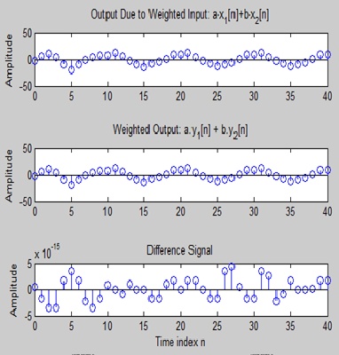
Yes this system is liner an if v add the both signal then its sum become zero..so both signals are equal.
Question #06
% Program P1_2 % Generate the input sequences
close all; clear all;
clc
n =0:40;
a = 2;
b = -3;
x1 = cos(2*pi*0.1*n);
s1=[x1 0].*[0 x1];
x2 = cos(2*pi*0.4*n);
s2=[x2 0].*[0 x2];
x = a*x1 + b*x2;
s=[x 0].*[0 x];
num = [2.2403 2.4908 2.2403];
den = [1 -0.4 0.75]; ic = [0 0]; % Set zero initial conditions
y1 = filter(num,den,s1,ic); % Compute the output y1[n]
y2 = filter(num,den,s2,ic); % Compute the output y2[n]
y = filter(num,den,s,ic); % Compute the output y[n]
yt = a*y1 + b*y2;
d=y-yt;% Compute the difference output d[n]
% Plot the outputs and the difference signal
dd=0:length(n);
subplot(3,1,1)
stem(dd,y);
ylabel('Amplitude');
title('Output Due to Weighted Input: a\cdotx_{1}[n]+b\cdotx_{2}[n]');
subplot(3,1,2)
stem(dd,yt);
ylabel('Amplitude');
title('Weighted Output: a.y_{1}[n] + b.y_{2}[n]');
subplot(3,1,3)
stem(dd,d); xlabel('Time index n'); ylabel('Amplitude');
title('Difference Signal')
D = y[n] - yt[n] not equal to zero so both are not equal..
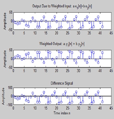
And the system is not linear.
Question #o7
% Program P1_3 % Generate the input sequences
close all; clear all;
clc
n = 0:40;
D = 10;a = 3.0;
b = -2;
x = a*cos(2*pi*0.1*n) + b*cos(2*pi*0.4*n);
xd = [zeros(1,D) x];
num = [2.2403 2.4908 2.2403];
den = [1 -0.4 0.75];
ic = [0 0];% Set initial conditions % Compute the output y[n]
y = filter(num,den,x,ic); % Compute the output yd[n]
yd = filter(num,den,xd,ic); % Compute the difference output d[n]
d=y- yd(D+1:41+D); % Plot the outputs
subplot(3,1,1)
stem(n,y); ylabel('Amplitude'); title('Output y[n]');grid;
subplot(3,1,2);
stem(n,yd(1:41)); ylabel('Amplitude');
title(['Output Due to Delayed Input x[n ', num2str(D),']']);
grid;
subplot(3,1,3);
stem(n,d); xlabel('Time index n'); ylabel('Amplitude');
title('Difference Signal');grid;
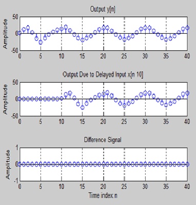
This iz time invariant system..and both signals are anot equal in sequence..
Question #08
% Program P1_3 % Generate the input sequences
close all; clear all; clc; n = 0:40; D = 10;a = 3.0;b = -2;
x = a*cos(2*pi*0.1*n) + b*cos(2*pi*0.4*n);
s=[n.*x 0]+[0 x];
xd = [zeros(1,D) s];
num = [2.2403 2.4908 2.2403];
den = [1 -0.4 0.75];
ic = [0 0];% Set initial conditions % Compute the output y[n]
y = filter(num,den,s,ic); % Compute the output yd[n]
yd = filter(num,den,xd,ic); % Compute the difference output d[n]
d=y- yd(D+1:42+D); % Plot the outputs
subplot(3,1,1)
stem(y); ylabel('Amplitude'); title('Output y[n]');grid;
subplot(3,1,2);
stem(yd(1:42)); ylabel('Amplitude');
title(['Output Due to Delayed Input x[n ', num2str(D),']']);
grid;
subplot(3,1,3);
stem(d); xlabel('Time index n'); ylabel('Amplitude');
title('Difference Signal');grid;
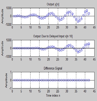
Yes the system is time invariant..


